Abaqus experiment with grid deformation and deflectometry
Let’s now go through the necessary steps for doing pressure reconstruction. First, we need to import the tools:
import recolo
import numpy as np
The example data can be downloaded from the recolo/examples/AbaqusExamples/AbaqusRPTs folder. The dataset corresponds to a 300 x 300 mm thin plate exposed to a sinusoidal pressure distribution in space and a saw-tooth shaped history in time.
mat_E = 210.e9  # Young's modulus [Pa]
mat_nu = 0.33  # Poisson's ratio []
density = 7700
plate_thick = 5e-3
plate = recolo.make_plate(mat_E, mat_nu, density, plate_thick)
We now set the pressure reconstuction window size. Note that as we here use noise free data on a relatively coarse dataset, a very small window size is used:
win_size = 6
Additive gaussian noise is added to the deformed grid images to mimic real world noise levels:
noise_std = 0.009
We now load Abaqus data:
abq_sim_fields = recolo.load_abaqus_rpts("path_to_abaqus_data"))
In this case, the deflection fields from Abaqus are used to generate grid images with the corresponding distortion. The grid images are then used as input to deflectomerty and the slope fields of the plate are determined:
slopes_x = []
slopes_y = []
undeformed_grid = recolo.artificial_grid_deformation.deform_grid_from_deflection(abq_sim_fields.disp_fields[0, :, :],
                                                                                abq_sim_fields.pixel_size_x,
                                                                                mirror_grid_dist,
                                                                                grid_pitch,
                                                                                img_upscale=upscale,
                                                                                img_noise_std=noise_std)
for disp_field in abq_sim_fields.disp_fields:
     deformed_grid = recolo.artificial_grid_deformation.deform_grid_from_deflection(disp_field,
                                                                                     abq_sim_fields.pixel_size_x,
                                                                                     mirror_grid_dist,
                                                                                     grid_pitch,
                                                                                     img_upscale=upscale,
                                                                                     img_noise_std=noise_std)

     disp_x, disp_y = recolo.deflectomerty.disp_from_grids(undeformed_grid, deformed_grid, grid_pitch)
     slope_x = recolo.deflectomerty.angle_from_disp(disp_x, mirror_grid_dist)
     slope_y = recolo.deflectomerty.angle_from_disp(disp_y, mirror_grid_dist)
     slopes_x.append(slope_x)
     slopes_y.append(slope_y)

slopes_x = np.array(slopes_x)
slopes_y = np.array(slopes_y)
pixel_size = abq_sim_fields.pixel_size_x / upscale
The slope fields are then integrated to determine the defletion fields:
# Integrate slopes to get deflection fields
disp_fields = recolo.slope_integration.disp_from_slopes(slopes_x, slopes_y, pixel_size,
                                                       zero_at="bottom corners", zero_at_size=5,
                                                       extrapolate_edge=0, downsample=1)
Based on these fields, the kinematic fields (slopes and curvatures) are calculated.
kin_fields = recolo.kinematic_fields_from_deflections(disp_fields, pixel_size,
                                                abq_sim_fields.sampling_rate,filter_space_sigma=10)
Now, the pressure reconstuction can be initiated. First we define the Hermite16 virtual fields:
virtual_field = recolo.virtual_fields.Hermite16(win_size, abq_sim_fields.pixel_size_x)
and initialize the pressure reconstruction:
pressure_fields = np.array(
[recolo.solver_VFM.pressure_elastic_thin_plate(field, plate, virtual_field)
                                                 for field in kin_fields])
The results can then be visualized:
import matplotlib.pyplot as plt
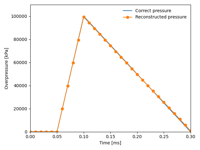
# Plot the correct pressure in the center of the plate
times = np.array([0.0, 0.00005, 0.00010, 0.0003, 0.001]) * 1000
pressures = np.array([0.0, 0.0, 1.0, 0.0, 0.0]) * 1e5
plt.plot(times, pressures, '-', label="Correct pressure")
# Plot the coreconstructed pressure in the center of the plate
center = int(pressure_fields.shape[1] / 2)
plt.plot(abq_sim_fields.times * 1000., pressure_fields[:, center, center], "-o",label="Reconstructed pressure")
plt.xlim(left=0.000, right=0.3)
plt.ylim(top=110000, bottom=-15)
plt.xlabel("Time [ms]")
plt.ylabel(r"Overpressure [kPa]")
plt.legend(frameon=False)
plt.tight_layout()
plt.show()
The resulting plot looks like this: